This post provides a primer to accompany and expand upon the tutorial on multiple regression in R. Watch Part 1 and Part 2 on YouTube. It is a work-in- progress—if you have feedback, please leave a comment.

Regression-based techniques, broadly speaking, are among the most powerful and useful tools available to the modern researcher, analyst, or data scientist. Why? I think it is in large part because they are so intuitive.

Have you heard a phrase along the lines of “the quickest route between two points is a straight line”? That phrase and its vicissitudes capture the idea that the optimal and simplest path from a point A to a point B is, in principle, a line. Similarly, one of the best and simplest ways to describe a relationship between variables is, in principle, a line.

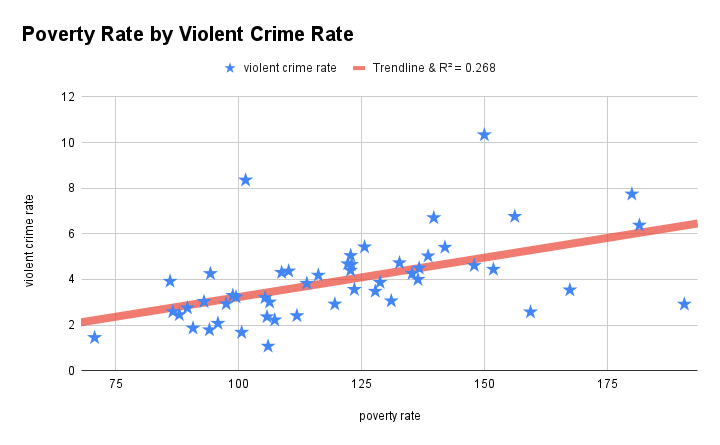
The chart above is called a scatterplot (an especially cheeky, patriotic one thrown together in Google sheets). Each “star” is a data point corresponding to a state in the United States. On the x-axis (horizontal-axis) is the 2020 poverty rate per 100,000 people (from U.S. Census Bureau); on the y-axis (vertical-axis) is the 2020 violent crime rate per 100,000 people (from FBI UCR program). The line goes by different names depending on context, but one name is the trendline. An apt name because it is a line…that captures a trend…

Without doing any math, I could have shown you the scatterplot on a piece of paper and said, “draw me a line from left to right such that each star is touching it or as close to it as possible”, and you likely would have drawn a line that resembles the trendline in the chart. This gets at a big idea in statistical modeling–virtually every estimation routine operates on the conceptual goal of minimizing the distance between “data points” and “trends”.

A trendline has two parts: An intercept (where the line starts on the y-axis) and a slope (what the line does as you look from left to right). My commute to work could be described with an intercept and slope: I start at my home about 15 miles from my office (intercept), and then drive in my car at about 45 miles per hour (slope). With those pieces of information alone, I could predict that 15 minutes after leaving home on my commute, I will be about 4 miles from work. Will that prediction be accurate for my commute on any given day? Maybe. Maybe not. Let’s say one day I am actually 5 miles away from work, rather than the predicted 4. This leads to another important component of regression equation beyond an intercept and slope: the residual or “error” term.

Dependent Variable = Intercept + Slope*Independent Variable + Residual

The residual term is probably one of the more persistently misunderstood aspects of the regression equation. One reason it is important is because it is used in the calculation of several important statistics, like standard errors. I think one source of misunderstanding stems from the word “error”. The word “error” usually connotes a mistake, but the residual “error” is an estimate of the variance of a variable in a population. Simply based on the fact that we are using information from a sample to draw a conclusion about a population means that there will be “error”, but it is a very specific kind of error, sampling error. It is does not (or at least should not) include other sources of error, like error due to unreliable measurement.

When you start with the idea that the residual term is supposed to capture sampling error (and not other sources of error), it is a little clearer why we make assumptions about it and why, when those assumptions are violated, our results can be biased.

The three main assumptions about residuals in traditional linear regression are that: 1) residuals are normally distributed, 2) residuals are homoscedastic (have a stable variance), and 3) residuals are independent. These all stem from the idea of taking simple random samples from a population. If you take a simple random sample from a population and estimate a parameter, the degree to which that estimate will match the true parameter is a function of variance and sample size.

In the real-world, I don’t think most researchers and analysts have data from true simple random samples in their day-to-day work. A fundamental reason checking assumptions is a recommended part of a routine is because we want to see if our data is even close to resembling what they would look like if they were from a true simple random sample. We’re often violating a premise of inferential statistics even when assumptions are met, but we learn the rules to break them baby!

A Gentle Introduction to Model Estimation and Assumption Diagnostics

The underlying logic of estimating a linear regression model using ordinary-least-squares estimation is surprisingly straightforward. I previously noted that: 1) estimation routines basically work by minimizing the difference between “trends” and “data points”, and 2) the residual term is a random variable that reflects sampling error. The smallest possible differences between a “trend” and “data points” would occur when the average difference is…zero! To “solve” a regression equation for a slope and an intercept, we treat the residual term like a continuous, random variable with a mean of zero.

Formally, the parameters are chosen such that the residual sum of squares is equal to zero. Written as a formula in a spreadsheet, it looks like this:

SUM((Predicted values – Observed values)²) = 0, where:

Predicted values = Intercept + Slope*Independent Variable

I do not think I am unique in how long it took me to realize what “least squares” actually meant. In looking at the scatterplot with violent crime rate and poverty rate, I said you could probably draw a trendline that would approximately match the estimated one. Without doing any math, you can intuitively draw a line such that the differences between the line and datapoints would be, on average, approximately zero. OLS estimation is essentially doing the equivalent. “Least squares” -> “smallest possible sum of squared residuals” -> zero.

(Normal Theory) Maximum likelihood estimation (MLE), another common routine for estimating regression models, works a bit differently than OLS. However, the conceptual goal is the same–choosing parameters such that the differences between the model and the data are at a minimum. I will be writing about MLE in later posts, so for this post I am going to focus on the OLS routine.

Let’s have a look at the residuals in our model of violent crime rates regressed onto poverty rates. The plot below is a histogram of the residuals (created using ggplot2 package in R). Do they look normally distributed?

Outside of what many would consider two outliers for different reasons (that’s Washington D.C. and Alaska on the far right), the residuals do appear to be approximately normally distributed with a mean of zero. One method of testing whether this assumption is called the “Jarque-Bera test” (Jarque & Bera, 1980), which tests the null hypothesis that skew and excess kurtosis are equal to zero (in a perfectly normal distribution, skew and excess kurtosis would be equal to zero). The results of that test indicated the null hypothesis should be rejected (p < .001).

I will temporarily sidestep the conversation to be had about how to proceed in a situation like this, but I will note that the results of the Jarque-Bera test are the opposite when outliers are removed. And on that note, I will completely sidestep the conversation to be had about outliers–at least in this post–but suffice it to say there are arguments both for and against excluding outliers.

The next plot is a scatter plot with poverty rate on the x-axis and the residuals on the y-axis, as well as a trendline. It provides a visual for inspecting residual heteroskedasticity. Basically, what you want to see is a horizontal trendline, as that indicates there is no relationship between the predictor(s) and residuals.

Residual heteroskedasticity can appear in multiple forms. One form of residual heteroskedasticity is linear heteroskedasticity, when residuals have a linear association with one or more predictors. However, just as a set of predictors could have linear, non-linear, interactive, indirect, etc., relationships with a dependent variable, so too could a set of predictors have complex relationships with the residual term. Tests for residual heteroskedasticity regress the residual term on predictors and specify different forms of the relationships. The “Breusch-Pagan test” (Breusch & Pagan, 1979) tests for linear heteroskedasticity, whereas White (1980) proposed a more general test with a full version including linear relationships, non-linear relationships (i.e., squared terms), and interactive effects. In this scenario with a single predictor, the only difference is whether the squared poverty rate is included or excluded. The results of both tests indicate that the null hypothesis of residual homoskedasticity should not be rejected.

The assumption of residual homoskedasticity is arguably one of the most critical assumptions because when it is violated, standard errors and, in turn, p-values will be biased. Some, but not all, of the other assumptions, like normally distributed residuals, can have negligible effects if violated or can be assumed a priori (e.g., you should know whether observations are independent before you even open a dataset).

Model Fit and Slicing the Pizza

In a way, I think modern inferential statistics can be summarized as capitalizing on basic mathematical properties. One big one is stupidly simple and is the equivalent of saying “you can cut a whole pizza into slices and then assign those slices to people; regardless of how you slice it, you still have one whole pizza.” Analogously, we can “slice” the variation of variable into portions and assign those portions to “people” (e.g., one or more explanatory variables). However, if we want to make inferences about a population, a lot of boxes have to be checked.

The trendline that best fits a given dataset can be calculated using OLS, but the extent to which we can meaningfully interpret that trendline as approximating something out there in the real-world depends on a lot of things. Beyond the three assumptions about residuals already mentioned, other notable mentions include perfect measurement and a correctly specified model. I like to focus on the latter because I think it has trickle-down effect and is within the control of the analyst. Residual heteroskedasticity, for example, can occur even in a regression model with data from a large, simple random sample from a population if the regression equation is simply wrong!

The fundamental “slicing” in a regression model estimated with OLS is delineating “explained variance” and “unexplained variance” in the dependent variable. The latter we have already tackled–it is the sum of squared residuals (differences between predicted and observed values). The other, also called the regression sum of squares, is the sum of squared differences between the predicted values and the mean of the dependent variable. The coefficient of determination, R², is the ratio of explained variation to total variation.

Of the many ways a model can be incorrectly specified, one way is mis-specifying the form of a relationship. Single predictor variable may have a relatively complex relationship with a dependent variable. For example, let’s consider the relationship between poverty rate and violent crime rate again, but now let’s additionally consider a poverty rate^2 term. A squared term means that a variable interacts with itself, which sounds strange, but it simply implies that the slope representing the relationship between poverty and crime might be slightly different, for example, in states with very high poverty rates. If you look at the chart, visual inspection would somewhat support the idea that when the poverty line surpasses 150 per 100,000, the relationship plateaus.

If we add the squared poverty rate term to the regression equation, the residual sum of squares decreases by about 4.69, the regression sum of squares increases by about 3.24, and R² increases by about .03. At this point, it is tempting to say that we have a more accurate model, which is technically true for our observed data. Sometimes researchers and analysts are not testing hypotheses about parameters and the entire goal can be to identify the model with the most accurate predictions. In that case, it is common to estimate several if not numerous models (e.g., using a machine learning approach) and compare the mean squared residual values (or “Mean Squared Error”). When you are interested in hypothesis testing, it is possible to test models against each other, with the null hypothesis being that the models provide an equivalent fit.

In this specific case, we can use ANOVA. As an overall test, it is typical to take the mean regression sum of squares (sum of squares/degrees of freedom) and divide by the mean residual sum of squares (again, sum of squares/degrees of freedom) to calculate an F-ratio. It is possible to use a similar approach to compare models by using differences in sum squares and degrees of freedom (e.g., by adding the squared term, we lose one residual degree freedom, so the difference in residual degrees of freedom between the models is one). The corresponding F-ratio in this case is 1.99 (p = 0.16) and would typically result in a failure to reject of the null hypothesis that the models provide an equivalent fit to the data.

The Cart, The Horse, and The Driver

In a previous post, I used the analogy of the cart, the horse, and the driver to describe the roles of design, analysis, and theory. My main point was that problems in statistical analyses are often rooted in theoretical and/or methodological problems. When I was starting as a researcher, I almost always viewed assumption violations or other “problems” as strictly statistical problems with statistical solutions. While that is possible and does happen, with increasing experience I realized I was often neglecting theory and/or design to some extent and that that was the source of the problem.

In this post, I jumped right into assessing the relationship between poverty rate and crime rate in 2020. If you think about it, this model does not make much sense. Implicitly, it draws on some theory proposing that crime is an outcome of poverty. Thus, it does not make theoretical sense to look at these rates in a single year as it inhibits temporal ordering. There is a mismatch between design (cross-sectional data) and analysis. Moreover, we could regress poverty rate onto crime rate and have a statistically equivalent model (think correlation). The extent to which we can assume the model is correctly specified is based on theory and design, and in this case, there is not much of a foundation for assuming our model is correct.

There are many “robust” approaches that can be used when one or more assumptions are violated. (I will be writing about them.) However, it is important to avoid being a hammer that only sees nails. If you run into an assumption violation, do not forget to consider the potential roles of the cart and the driver. Horsepower is admittedly more exciting, but it alone is rarely sufficient to get from point A to point B.

References

Breusch, T. S., & Pagan, A. R. (1979). A simple test for heteroskedasticity and random coefficient variation. Econometrica, 47(5), 1287-1294.

Jarque, C. M., & Bera, A. K. (1980). Efficient tests for normality, homoscedastity and serial independence of regression residuals. Economic Letters, 6, 255-259.

White, H. (1980). A heteroskedasticity-consistent covariance matrix estimator and a direct test for heteroskedasticity. Econometrica, 48(4), 817-838.