In this next installment of “Monte Carlo Mondays”, I want to illustrate another use of the Monte Carlo method. In the first installment, I used the Monte Carlo method to conduct an experiment to answer methodological questions. Beyond answering methodological “what ifs”, another application of the Monte Carlo method I think is useful is simulating the null distribution.

Several “state of the art” approaches involve generating a distribution, like testing indirect effects using the product-of-coefficient method and testing the impact of a policy change using the synthetic control method. The latter is in the vein of what I will describe in this post, where the goal is generating a distribution representing the counterfactual. The approach offers control and flexibility, and, in my view, can be especially useful for “small-n case studies”, what John Eck (2006) once described as the bologna sandwiches of research design (though I prefer to call them ham sandwiches). The two main components of it are conjunctive analysis of case configurations (CACC) and Fisher’s exact test.

Conjunctive Analysis of Case Configurations

In the discipline I was trained in, criminology and criminal justice, CACC was coined and popularized by Miethe et al. (2008). Without getting into all the background and nitty-gritty details, I think the simplest way of describing it is contingency tables: the sequel. If you have a bunch of discrete independent variables and a discrete dependent variable, you can create a table where each column is a variable and each row represents a unique profile of attributes across those variables. There are parallels to other approaches where the goal is capturing underlying subpopulations (e.g., mixture modeling).

Notably, I think you could just employ some sophisticated mixture modeling technique in many cases, but the tenability of that in a “ham sandwich” scenario is questionable. And I have a soft spot for ham sandwiches.

Often when we classify subpopulations we also want to test if there are meaningful differences across those subpopulations in some outcome. In a ham sandwich scenario, employing Fisher’s exact test in addition to CACC is one option that I find useful.

Fisher’s Exact Test

A conventional approach to examining a relationship between two discrete variables is to create a contingency table and use a chi-square test of independence. This approach is flawed with small samples. The rule-of-thumb I learned was cell sizes less than 5 = bad. Conventional hypothesis testing involves calculating a test statistic and assuming it comes from a certain sampling distribution (e.g., a chi-square distribution). With small counts in cells, the “chi-square” you calculate based on observed and expected counts in contingency tables is not actually chi-square distributed, so the p-values will be biased.

Fisher’s exact test does not require a minimum cell size. It is an “exact” test because the idea is that you create a probability model and use it to determine the exact probability of events if the null hypothesis were true. Not only can it be applied in a small-n scenario, but it is also useful in the CACC context because it can be used to test the probability of a given profile having a certain outcome if the profile was present by random chance. With a contingency table we want to know if variables are independent, in what is called the “truth table” in CACC terminology, we want to know if combinations of variable attributes are independent from an outcome.

The Case of Case Outcomes

For most of my time in academia, I was interested in sentencing outcomes in death penalty cases. Capital cases are rare, particularly at lower levels of analysis like the county-level and when the time period is limited. Compiling and coding records, even when they do exist, takes a lot of resources. Moreover, rarely are there incentives for doing it.

The overarching advantage of what I’ll label CACCf in a ham sandwich, small-n case study like cross-case comparisons in rare cases in a state or county is that it is an elegant combination of elements traditionally found in qualitative and quantitative research. Coding attributes of cases and adopting a more idiographic perspective on causation tends to be qualitative, and statistical inference is quantitative.

In this particular case study, I was interested in the “new death penalty”, life without parole (LWOP). At the time, I was an assistant professor at a university in Illinois. Illinois is similar to other states that, after abandoning the death penalty, more-or-less retained the sentencing scheme for life without parole. I and my colleague, Logan Yelderman, argued in a paper that death sentences are basically the result of legal factors in cases that, by law, are supposed to circumscribe sentencing decisions (Gregg v. Georgia, 1976). Saying that evidence is the main factor that drives sentencing decisions is not novel by any stretch, and even one of our provocative arguments was turning a question posed by Richard Wiener in his reflection on George Baldus and colleagues’ study of Nebraska capital cases into a declarative statement:

“…specific aggravating circumstances activate automatic, perhaps inescapable affective reactions in judges, prosecutors, and very likely jurors, which result in immediate, nondeliberative judgements of deathworthiness.”

Wiener (2002, p. 765)

In our account, specific types of aggravating legal factors in capital case, like multiple victims and sexual assault, can trigger moral intuition and emotion and result in rationalizing a death sentence. We also think this generalizes to LWOP cases, particularly in a jurisdiction like Illinois where the same statutory factors that once justified a death sentence now justify LWOP for murder.

I started by downloading publicly available admissions data from the Illinois Department of Corrections for 2018, 2019, and 2020. I then turned to the Illinois Courts website to identify appellate court opinions associated with these cases; I also searched for news articles covering the cases. Ultimately, I had a sample of 22 LWOP cases, 15 of which were mandatory LWOP and 7 of which were discretionary LWOP. I also created a comparison group of 7 murder cases that resulted in “virtual” life sentences (e.g., 80 years).

Based on theoretical perspectives, I wanted to see how defendant characteristics, specifically race, age, gender, and certain legally and morally aggravating factors (e.g., whether there was evidence of sexual assault) related to sentencing outcomes. The admissions data had demographic information, and court opinions and/or news sources had the aggravating factors.

I first examined whether profiles based on race, age, and gender distinguished between sentencing outcomes. I started with mandatory v. discretionary LWOP. Of the 8 possible configurations–each variable was binary (e.g., age was 35 years old or younger or not)–5 were observed. Two of the profiles–younger, non-White men and older, non-White men–accounted for almost 70% of cases, and more than 65% of cases that fit these profiles resulted in a mandatory LWOP sentence.

To simulate the null distribution, I generated random variables based on descriptive statistics. For example, about 91% of defendants were men, so I randomly sampled from a Bernoulli distribution with a probability of 91% to generate the gender variable. I repeated this process 10,000 times to generate a distribution of expected counts under the null hypothesis. I could then calculate the probability of the observed count given the distribution under the null hypothesis. Below is the null distribution for the younger, non-White men profile with the observed count of cases in the profile that resulted in a mandatory LWOP sentence.

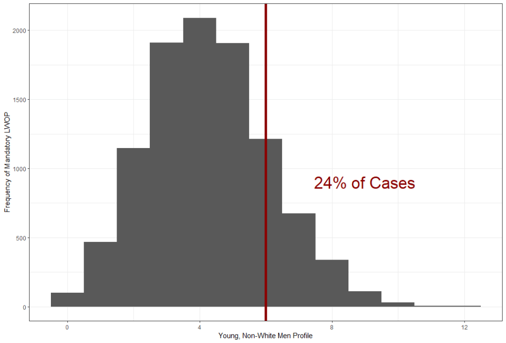
Under the null distribution, there is an almost 1 in 4 chance that 6 or more cases with the young, non-white men profile would result in a mandatory LWOP sentence. With a conventional alpha level of .05, this indicates a failure to reject the null hypothesis. There was a failure to reject the null hypothesis for this profile, but for all other profiles as well. The conclusion would be that the probability of a defendant convicted of at least one murder and eligible for LWOP receiving a mandatory LWOP sentence is independent of age, race, and gender (as crudely measured here).

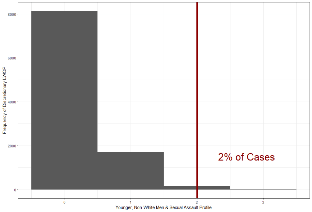
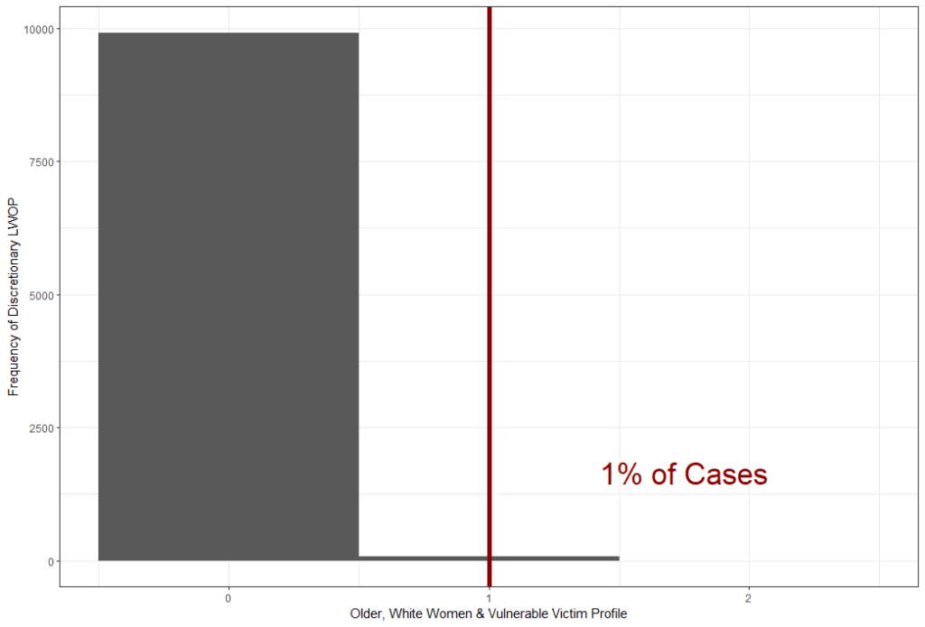
The same story played out for the comparison of discretionary LWOP to virtual LWOP. However, when I added aggravating factors, multiple victims (i.e., murder of one victim and attempted murder of another), sexual assault, and “vulnerable” victims (i.e., children or senior citizens), a different story played out. Three profiles were statistically significant–two if two-tailed tests were used. The charts below are for the younger, non-White men and sexual assault profile, the older, White women and vulnerable victim profile, and the older, White men and vulnerable and multiple victims profile.

Discussion & Conclusions

Some have suggested that demographic disparities in sentences are better understood as “case-effects”. One general, contemporary view is that, to the extent that there are stereotypes associated with demographic characteristics, their influence is more likely to occur in early stages of the justice process where discretion is less constrained. Discretion at sentencing technically does not exist in some cases–in Illinois, being convicted for multiple murders makes an LWOP sentence mandatory. When there is discretion, it is often substantially constrained. From this perspective, it makes sense that profiles based on (crude) measures of age, race, and gender would be independent of sentencing, but profiles based on age, race, and gender in combination with “gut-punching” legal factors are not independent of discretionary LWOP sentencing.

This is a ham sandwich study, but again, I have a soft spot for ham sandwiches. They can be “theoretically generalizable”, which is basically to say that, if you have a good rationale, your theoretical conclusions may extend to other instances in which that rationale is applicable. In a hypothetical alternative Illinois, I might not replicate the findings, but I do not think it would be surprising to find that demographic characteristics in conjunction with certain types of evidence were not independent of discretionary LWOP sentences.

CACCf is neat way to derive insights from ham sandwiches. And it’s not that hard to do–you could actually do it in Google sheets or Excel. I focused on case outcomes here, but CACCf has been and could be applied to other things. I think it is a particularly good approach when you have several discrete variables, a small sample, and use an “exploratory” method with a “confirmatory” approach.