A colleague of mine recently brought up the “rule of ten”. Like a lot of so-called “rules”, it is actually a heuristic and was never proffered as a rule (Peduzzi et al., 1996). And like any heuristic, it is at best generally helpful albeit misleading. The rule states that, for a binomial, logistic regression model, the maximum number of predictors is equal to the minimum number of events divided by 10. In other words, the event per variable ratio should be 10 to 1. For example, if your sample size was 100 total cases and your outcome had a 90/10 split, according to the rule of ten you could have a maximum of one predictor (10 events/10 = 1).

To start the “Monte Carlo Mondays” series, I decided to investigate the rule of ten. Not in general, but in a relatively small-n and single-predictor scenario. My thinking is that this represents–not a worst-case scenario–but a mediocre one. The overarching question in this narrow scenario is: How does the base rate/event per variable rate under different effect size conditions affect coefficients, standard errors, and p-values? Here is a how I set up my Monte Carlo experiment:

Sample size (n) = 100

Simulations (k) = 10,000

Base rate (%events) = 1%, 3%, 5%, 7%, 9%, 11%

Effect size (r) = Small (-.10), medium (-.20), or large (-.50)

For the dependent variable, I initially generated a continuous, normally distributed variable with a mean of zero and a variance of 1, and then used cut-points corresponding to base rates to create six dependent variables. The independent variable was generated as a continuous, normally distributed variable with a mean of zero and a variance of 1.

SMALL EFFECT SIZE

Intuitively, I suspected that this scenario would show the largest effects of base rate because generally small samples + small effect sizes = problems.

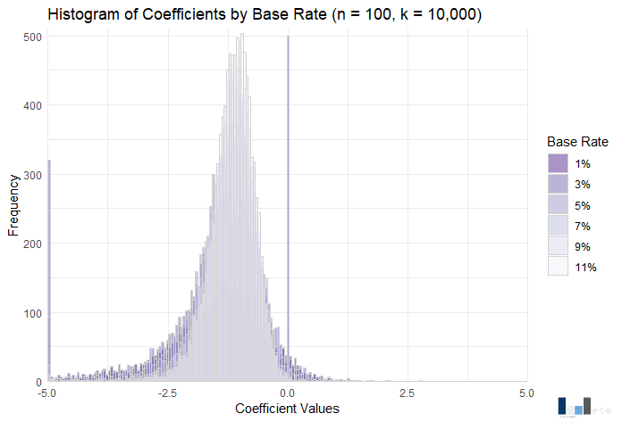
The chart above shows the distributions of the coefficients by base rate (constraints imposed for clarity on this and subsequent charts). One take-away from visual inspection is the relationship between base rate and variance. That is, the variance increases as the base rate decreases. The other take-away, supported with additional calculations, is that the coefficient estimate, on average, decreases in magnitude. Notably, however, the median was virtually the same for each base rate, with the exception of 1%. None of the distributions are normal, but the distribution moves closer to normality as the base rate increases. Kurtosis, specifically, decreased dramatically (e.g., at 5% base rate, kurtosis = 3,820.28; at 9% base rate, kurtosis = 4.88).

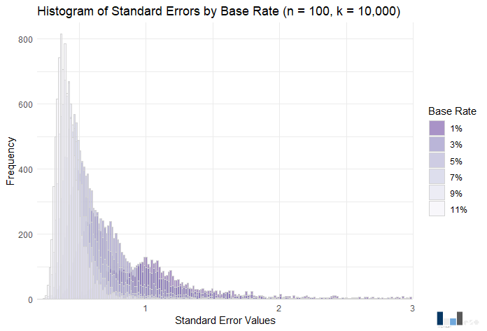
The distribution of coefficients implies problems for hypothesis testing. In testing coefficients, it is commonly assumed that the sampling distribution of the coefficient is normal. Hypothesis testing or not, the high variance and “thick tails” in the distribution mean accurate estimation is difficult. Now let’s take a look at standard errors.

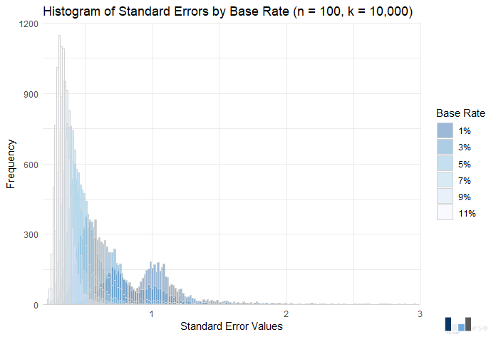
Some trends in standard error distributions are similar to that of coefficients: The variance and average standard error decrease as the base rate increases. Unlike coefficients, the median also decreases as the base rate increases, which can be seen in the contrasting distributions.

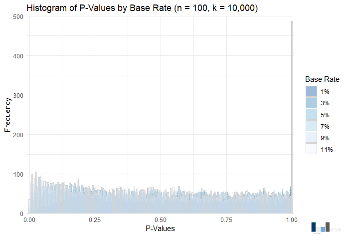
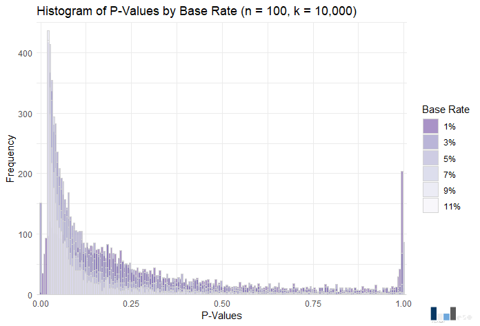
Given the distributions of the coefficient and standard error, you will likely not be shocked by the distributions of p-values. Power is abysmal across the board, ranging from .01 (1% base rate) to .08 (11% base rate).

MEDIUM EFFECT SIZE

The results for the small effect size more-or-less matched my intuition. If your goal was testing the null hypothesis that the coefficient is zero, you are basically out of luck. If your goal was simply to obtain an accurate estimate, the accuracy of the estimate would depend on the rarity of the event. Now let’s look at the medium effect size scenario.

The take-aways from this coefficient histogram are similar to the last (e.g., variance decreases with base rate). Let’s check out standard errors.

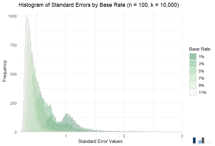
Here again the take-aways are similar to the last. What about p-values?

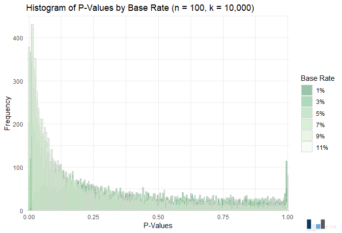
Alas, a visual contrast! The distribution of p-values for the small effect size looked nearly uniform, whereas here we see something that somewhat resembles a typical p-curve. Power exhibits much greater range across base rates, ranging from .03 (1% base rate) to .41 (11% base rate). The key distinction between the small and medium effect size conditions appears to be that a medium effect size augments the relationship between base rate and power.

Large Effect Size

What do you think the results of the large effect size scenario will be? The one that jumps to my mind is that power might start to get close to a traditionally accepted value of .80. Let’s look at all the charts and see what conclusions we can draw.

Visually, not much to write home about. However, the power range again increases, this time from .09 (1% base rate) to .85 (11% base rate). The rule of ten appears particularly applicable to power in this case, as at a 9% base rate power is just below .80 at .79.

Conclusions

With a fixed sample size of 100, power is heavily influenced by the joint effects of effect size and base rate, while the accuracy of estimates is influenced by base rate. To unpack the role of base rate more, consider the following:

Grand Average by Base Rate (1%, 3%, 5%, 7%, 9%, 11%)

Coefficient: -16.62, -4.23, -1.68, -.93, -.79, -.66

Standard Error: 14,053.27, 1,9860.29, 316.37, 55.98, 12.35, 0.85

P-Value: .63, .37, .29, .27, .24, .22

Average of Medians by Base Rate (1%, 3%, 5%, 7%, 9%, 11%)

Coefficient: -.34, -.72, -.70, -.68, -.66, -.64

Standard Error: 1.37, 0.69, 0.52, 0.45, 0.40, 0.36

P-Value: .68, .28, .22, .19, .18, .17

I show both grand average and average of medians because the comparisons are informative. Low base rates tend to come with extreme values and in turn some of the average coefficients and standard errors are outrageous. In contrast, the average of the medians shows surprising consistency at roughly 3-5% and higher. In short, there is a small chance your model would basically be uninterpretable with a base rate/event per variable rate under 10%, but there is a surprisingly decent chance your model would not be a pile of flaming hot garbage.

So what’s the verdict on the rule of 10 in this contrived scenario? In my view, the results suggest that the rule of 10 is a good heuristic to use if the goal is hypothesis testing and you expect a relatively strong effect. Outside of that, it is probably still a decent heuristic to keep in the back of your mind. I would not call it a good “rule”, as that implies legitimacy, but if you used it to inform, for instance, planning decisions, it would help more than hurt.

Want to see the R code? Shoot me an email at westdesignandanalysis@gmail.com

References

Peduzzi, P., Concato, J., Kemper, E., Holford, T. R., & Feinstein, A. R. (1996). A simulation study of the number of events per variable in logistic regression analysis. Journal of Clinical Epidemiology, 49(12), 1373-1379. https://doi.org/10.1016/S0895-4356(96)00236-3